Chapter 5 Broad use cases for genomic epidemiology
In this chapter we describe thematic areas of genomic epidemiological analysis for public health investigations. For each of these areas, we provide concrete examples of the types of questions that fall within these topical areas, the fundamental theoretical principles that you will draw upon to investigate those questions, and different sampling schemes and analysis methods for investigating those questions. This chapter is pertinent to most readers, as it describes the public health utility of different genomic epidemiologic analyses. Additionally, readers engaged in building genomic epidemiological capacity or in performing genomic epidemiology themselves will benefit from the descriptions of how to design, analyze, and interpret various genomic epidemiological investigations.
5.1 Assessing linkage between cases
5.1.1 What kinds of questions fall into this topic?
Both of these cases have similar reported exposures. Is that common exposure the likely source of both infections?
I have multiple detections of disease in the workplace. Is workplace transmission occurring, or were unrelated community-acquired infections detected at the same time?
I have multiple cases that were assigned the same Pango lineage. Are these cases closely-related?
There is an outbreak going on in our prison system, and there are also cases in our intake jails. Are infections in intake jails contributing to prison outbreaks?
I have two detections of a variant of concern from the same week, and I’ve never seen that variant in my jurisdiction before. Do these cases represent community transmission of the variant of concern, or are these cases independent introductions?
I’ve detected two cases of a disease in the same household. Is this an instance of household transmission, or did the cases contract the disease separately outside the home?
5.1.2 Fundamental principles
As a pathogen, let’s say a virus, circulates in a population, it infects different people. During those infections, the virus replicates, making errors as it copies its genome for packaging into progeny virions. While different pathogens make errors at different rates, and we may see substitutions in consensus genomes at different rates (see Chapter 3 - mutations versus substitutions), this principle means that pathogen genome sequences will accumulate changes over the course of an outbreak. This process also means that cases separated by a minimal amount of transmission will generally have more genetically similar infections, while cases that are separated by large amounts of transmission will typically have more genetically divergent infections.
5.1.3 What kind of sampling do you need to answer the question?
When you are looking at the pathogen genome sequences of two infections you are not extrapolating from those data to a broader understanding of the outbreak as a whole. Therefore, you can assess possible linkages between cases using sequences collected through either a targeted sampling scheme or a representative sampling scheme. That said, it remains important to include contextual sequence data in your analysis, as described in Chapter 3 and as shown in Figure 5.1 below.
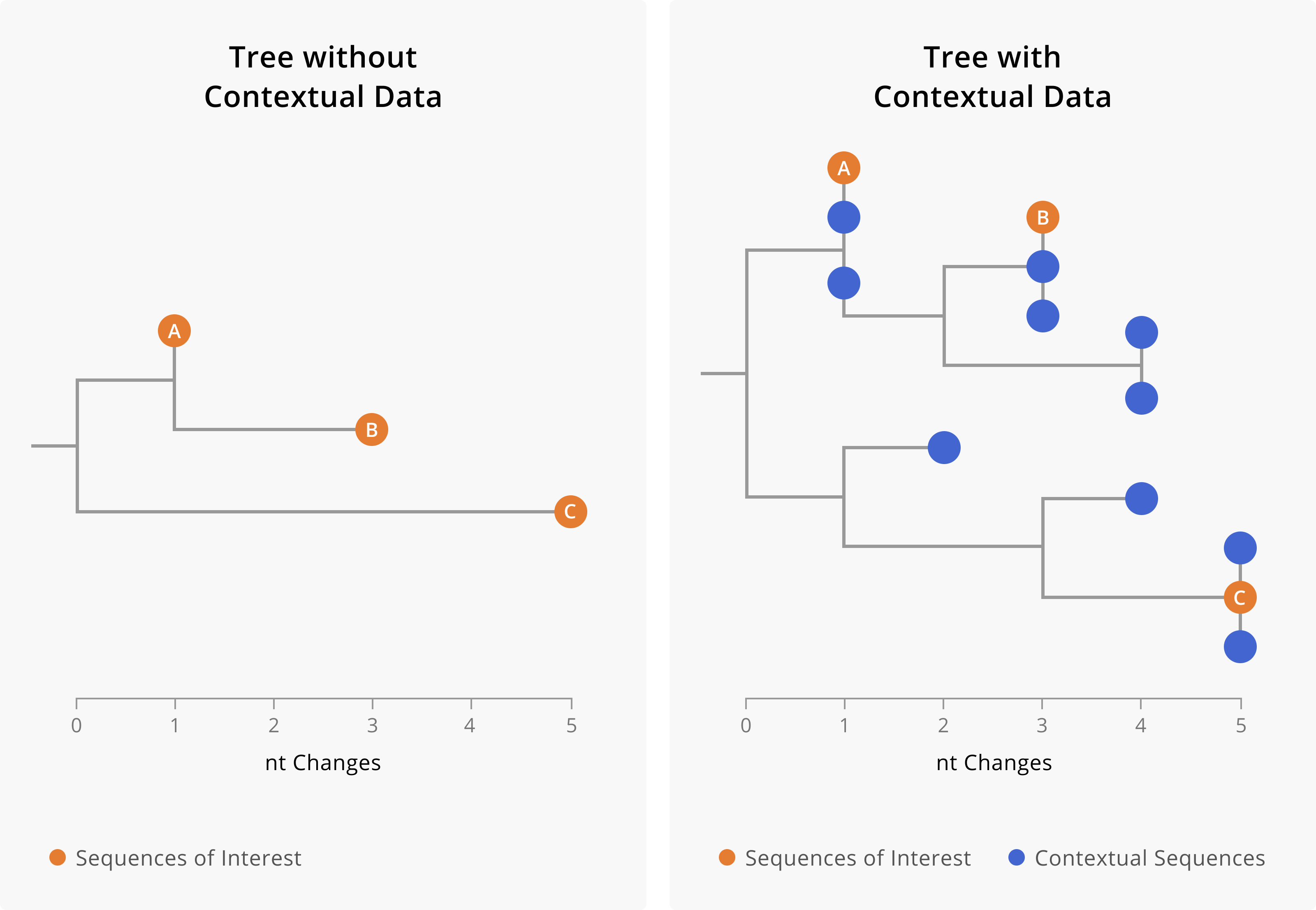
Figure 5.1: A toy example showing the importance of including contextual data when assessing linkage between cases. On the left-hand side is a phylogenetic tree including only three samples of interest. On the right-hand side, we show a phylogenetic tree of the same three samples of interest (orange tips) along with closely-related contextual data (blue tips). The addition of contextual data clarifies the relationships between the samples of interest. In the tree on the left, we might assume that A and B are related cases, since they both share a mutation and are only two nucleotides diverged from each other. However, the addition of contextual data (blue) provides a more nuanced picture. We see that samples of interest A and B are in fact more closely related to contextual sequences than they are to each other. This could mean that A and B are not directly epidemiologically-linked, or it might mean that A and B are both part of a larger transmission chain captured by the contextual sequences. Furthermore, contextual data can make it more clear when samples are diverged. While we can see substantial genetic divergence between sample C and samples A and B in the tree on the left, the addition of contextual data makes it more clear that C is unrelated to samples A and B.
5.1.4 What tools or approaches can you use to answer the question?
To investigate questions of linkage you will need a way to compare and summarize the genetic similarity between cases of interest. There are multiple methods for summarizing genetic distances between samples, but we generally recommend using tree structures such as phylogenetic placements or phylogenetic trees (see Chapter 7 for more details) when assessing sequence similarity between samples.
While it is technically possible to build a tree structure with just your samples of interest, we caution against doing this, as the addition of other contextual sequences usually makes the relationships between your samples of interest more clear. Furthermore, in the case that your samples of interest are not genetically similar to each other, the presence of contextual sequences allows you to see other samples that they are closely-related to (Figure 5.1).
Both phylogenetic placements and phylogenetic trees will provide a tree structure for assessing similarity between samples of interest. However, during public health investigations, our questions about the genetic similarity of samples of interest are usually limited in scope and we need answers quickly. When rapid situational awareness is more important than a richer analysis, we recommend performing a phylogenetic placement. If after performing a phylogenetic placement you have further descriptive epidemiological questions about the samples, then we recommend following-up a phylogenetic placement with inferring a phylogenetic tree.
5.1.5 Caveats, limitations, and ways things go wrong
As discussed in Chapter 3, genomic data are powerful for ruling linkage out, but less powerful for unequivocally ruling linkage in. Furthermore, except in rare cases, you cannot infer the directionality of transmission from sequence data alone when you have highly genetically-similar consensus genomes. This principle is probably clearest when cases have identical genome sequences, since if all of the sequences are the same there’s no genomic signal for directionality. However, we caution that directionality is still challenging to infer accurately even when some genomes are slightly diverged. As an example of this issue, in Figure 5.2 we illustrate two different transmission patterns that yield the sample phylogenetic tree topology. In the first scenario, we have a person-to-person transmission pattern, where directionality is A to B to C to D. In the second scenario we instead have a superspreading event, in which individual A directly infects person B, person C, and person D. Despite having different transmission patterns, the genetic divergence trees are identical. This example shows how challenging it can be to disentangle genetic diversity accrued during person-to-person transmission from within-host diversity that is transmitted when an index case infects multiple secondary cases.
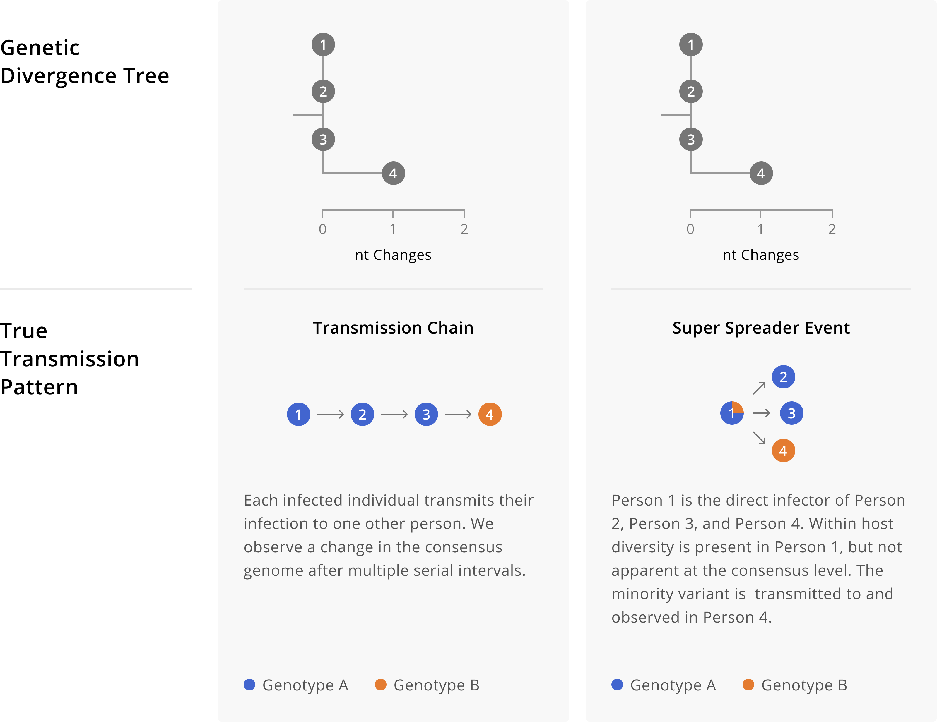
Figure 5.2: Different transmission patterns between individuals A, B, C, and D can yield identical genetic divergence trees. On the left we show a transmission chain in which individual A infects B, who infects C, who then infects D. Depending on the evolutionary rate of our pathogen, we may not see mutations arise in every single consensus genome. Indeed, here we see that the sequences from individuals A, B, and C are identical. Thus without knowledge of the true transmission pattern, we would not be able to detect the directionality of transmission between those three individuals. Furthermore, while one might initially think that directionality for individual D is possible to infer, comparison of the scenarios on the left and right show how directionality can become convoluted by within-host diversity. On the left, individual D’s consensus sequence shows an additional nucleotide change on top of the background genotype of A, B, and C, which was accrued over the process of transmission between individuals. In contrast, on the right that same pattern of diversity is present within individual A’s infection. Then, during a superspreading event in which A infects individuals B, C, and D directly, that within-host diversity is captured at the consensus level of the secondary infections. These toy trees are consistent with still more additional true transmission patterns that are not enumerated here. As an exercise you might want to try sketching additional possibilities out.
Additionally, in much the same way that contextual data may change your understanding of linkage between cases, lacking sequences from infections may also change your interpretation of linkage. When assessing linkage between cases, we recommend keeping your sampling frame in mind. If you’re assessing linkage between two samples collected through representative surveillance, then consider what proportion of cases you have sequence data for. If you sequence only a small proportion of cases, then there may be intervening cases along a transmission chain that go unsequenced, and therefore do not appear in a phylogenetic tree. In that case, genetically-similar samples could be part of the same transmission chain, but not necessarily directly epidemiologically linked.
Finally, some molecular epidemiological methods suggest using SNP distances and thresholds for ruling cases into the same outbreak or categorizing them as belonging to different outbreaks. While we understand how thresholds can make decision making easier, we generally discourage using SNP thresholds. This is because using SNP thresholds reduces the granularity of the data; they make a binary assessment (in or out of outbreak) when in fact the data are continuous (0, 1, 2, 3 … SNPs separating two sequences). While reducing the data down to a single binary outcome does make assessment easier, it does so by hiding nuance and uncertainty, which is critical for making epidemiologic inferences and assessing your confidence in them. Furthermore, making genetic distance into a binary call results in a loss of information. Pathogens accrue mutations at specific evolutionary rates, thus the actual count of differences between two sequences provides a quantitative estimate of how related or unrelated two sequences are.
5.2 Exploring relationships between cases of interest and other sequenced infections.
5.2.1 What kinds of questions fall into this topic?
Is my outbreak linked to other outbreaks elsewhere?
What other samples are closely related to my samples of interest?
5.2.2 Fundamental principles
Exploring relationships between cases of interest and other sequenced infections relies on the same principles as discussed in the previous use case (Assessing linkage between cases). The reason that we have separated these concepts within this handbook is not because the principles underlying these concepts are different, but rather because the sequences you are considering in your analysis will likely come from different populations. In the previous use case, public health practitioners are seeking to use genomic epidemiology to understand epidemiologic relationships between individuals within their own community, or wherever they have jurisdiction. In contrast, in this use case we describe why and how to explore relationships between your samples of interest and sequenced infections from other communities and regions.
5.2.3 What kind of sampling do you need to answer the question?
Within this broad use case, a question of interest centers around exploring possible links between your own cases (or outbreaks) and cases or outbreaks occurring in other communities. Contextualizing your own transmission in this way brings up a key concept and challenge; if you are looking for linkage with transmission in other contexts, then you want access to sequences that accurately capture the full scope of pathogen diversity circulating in those other contexts. This means that while you can select your own cases of interest in a way that aligns with the question you’re investigating, you typically need contextual data from other jurisdictions that has been sampled representatively. When sampled representatively, contextual data provide a more accurate summary of the circulating pathogen diversity in those other areas. When available sequence data from other regions accurately summarizes their own outbreaks, you can have greater confidence that you are accurately capturing the true presence or absence of cross-jurisdictional links.
This concept brings forth a few important considerations. Firstly, the need for representatively sampled contextual data is one of the reasons why we need broad, baseline genomic surveillance programs. In such programs, sequencing is performed at random, without regard to specific clinical presentations, performance on diagnostic assays, or public health questions. Representative sequencing is done partially for the common good; everyone will need contextual data from other communities or populations at some point. This principle is why we encourage groups building genomic surveillance systems to perform some degree of representative sequencing beyond their targeted outbreak sequencing. Furthermore, this rationale is also why annotating those sequences as representatively sampled surveillance specimens is a critical part of genomic surveillance data management.
5.2.4 What tools or approaches can you use to answer the question?
To answer these types of questions, we recommend phylogenetic approaches that summarize the genetic relationships between samples on a tree structure. Currently, there are two primary ways to infer a tree structure that includes your cases of interest: phylogenetic placements and phylogenetic trees. While the output of these two types of analyses may look similar, they are performing different processes. Each of these tree structures, as well as tools for performing phylogenetic placements and inferring phylogenetic trees, can be found in the “Tools and methods” chapter.
As an additional layer to building a phylogenetic tree, genomic epidemiologists will frequently investigate cross-community outbreak linkage using phylogeography. Phylogeographic analyses take in geographic information about where sequences were sampled and probabilistically reconstruct where ancestral pathogens in the tree likely circulated. More information about phylogeography and implementing phylogeographic analyses is given in the “Tools and methods” chapter.
5.2.5 Caveats, limitations, and ways things go wrong
While designing and maintaining representative sampling within your own jurisdiction can be challenging, influencing how sampling occurs externally is close to impossible. Variability in access to resources often leads to variability in which communities have pathogen genomic representation, which can directly impact your own inferences. While resourcing broad genomic surveillance programs at higher levels of jurisdictional authority (e.g. nationally) and clear annotation of representatively-collected data can mitigate this issue, the lack of control that you’ll generally have surrounding which contextual data actually exist publicly means that you should exercise some caution in interpreting your findings. This does not mean all is lost! For many investigations, genomic epidemiologists have simply analyzed whichever sequences existed or could be generated. And despite such non-ideal sampling, those analyses have still contributed greatly to our understanding of a pathogen’s epidemiology. We simply recommend recognizing that the data you have access to may be incomplete or biased, and that your interpretations may change upon the addition of more data.
As the amount of publicly-available sequence data increases, you may find yourself shifting from including all contextual sequences that you can find to having to choose which contextual data to include. This will be true in particular for phylogenetic tree-based analyses, where there is a practical limit on the number of sequences you can include. For guidance on how to choose which contextual data to include, please refer to that section within the “Tools and methods” chapter.
5.3 Estimating the start and duration of an outbreak.
5.3.1 What kinds of questions fall into this topic?
Our syndromic surveillance system isn’t as sensitive as we would like, and we aren’t sure how long we’ve had circulation of this pathogen in our community. When was this pathogen introduced into our community, and how long has it been circulating for?
We received reports of some initial cases of a disease, but we weren’t able to confirm an outbreak until later. Did this outbreak begin around the time of those initial case reports?
We had an outbreak in a congregate living facility, and we believe that we brought it under control, but we continue to have sporadic cases in the facility. Is the same outbreak still ongoing?
5.3.2 Fundamental principles
Genomic data are useful for estimating the timing of epidemiologic events in a few different ways. Firstly, estimating the timing of disease circulation from genomic data can be more accurate when the disease in question causes large numbers of asymptomatic infections or mild cases that do not seek treatment. In these scenarios, surveillance systems may only start to record cases once a sufficient number of infections have occurred to produce a subset of more severe cases that seek care or diagnostic testing. In contrast, even when an infection is asymptomatic or mild, viral replication will occur, leading to mutations that may be carried forward during transmission. In this way, a record of the infection can be left in the pathogen genome even when the infection does not rise to a sufficiently symptomatic level to be a recorded case. Furthermore, since genomic data can enable you to resolve distinct but concurrent outbreaks, temporally-resolved phylogenetic trees can provide cluster-specific estimates of timing. This feature is particularly useful once you have ongoing transmission, and the emergence of distinct clusters (such as the emergence of a new variant) may not be apparent within an epidemiologic curve.
In Chapter 3 we introduced molecular clocks, which represent the average rate at which a particular pathogen evolves. When we know on average the rate at which genetic diversity accumulates, we can take an observed amount of genetic diversity and ask: “How long would it have taken to accumulate this much diversity?” When we are looking at the genetic divergence between sequences sampled from the same outbreak or epidemic, calculating how much time was needed to generate that diversity provides an estimate of when that outbreak or epidemic likely started.
We generally investigate this type of question using a temporally-resolved phylogenetic tree, and we frame the question as “What is the time to the most recent common ancestor of these sequences?” Or, “When did the most recent common ancestor of these sequences likely circulate?” When sequences are genetically similar, little evolutionary time has passed, and the ancestor from which those sequences are descended will be more recent. When sequences are very diverged, a large amount of evolutionary time has passed, and the ancestor of the sequences of interest will have existed further back in time.
Every internal node within a phylogenetic tree represents an ancestor and will have an attached date. So, which internal node should you look at? Typically, the ancestral sequence that you are For example, if you are interested in estimating when an outbreak in a skilled nursing facility began, then the internal node that you would look for is the youngest node in the tree from which all SNF samples descend. Or if you are interested in when Zika virus likely arrived in the Americas, then you would look for the ancestral node from which all Zika virus genomes collected across all countries in the Americas descend.
5.3.3 What kind of sampling do you need to answer the question?
In order to estimate the molecular clock accurately, you will need genome sequences collected over longer time spans. The reason for this is fairly simple; it is very hard to accurately estimate the slope of a line when the only data points you have come from a single cross-sectional sample. In contrast, data points collected over time allows you to see much more clearly how genetic diversity and time correlate, thereby providing more consistent and accurate estimates of the evolutionary rate. Ideally your serial samples used in estimating the molecular clock should be sampled representatively. These serially-sampled sequences can either be sequences you generated, or they can be publicly available contextual sequences.
Once you have your estimate of the evolutionary rate, the samples of interest (whose ancestor you would like to date) can be sampled either representatively or in a targeted fashion, in accordance to your question of interest. If you are interested in when a localized outbreak began, then you may want to intensively sample and sequence infections that occur within that particular facility or setting. However, when the event that you would like to date has yielded many sequenced samples, it is best to sample the sequences representatively. For example, if I would like to estimate when SARS-CoV-2 was first introduced to California, I should select a representative sample of sequences from the entire state of California, and estimate when their ancestor likely circulated. While in theory I could perform targeted-sampling of the entire state of California and sequence every positive case, in reality that would be completely infeasible. Thus, to accurately estimate how much time was necessary for Californian viral diversity to accrue, I must have a representative sample of Californian SARS-CoV-2 diversity. If my sample is not representative, then the date that I infer will represent when the ancestor of the sample that I have.
5.3.4 What tools or approaches can you use to answer the question?
Using the molecular clock to translate the branch lengths of trees from genetic divergence (evolutionary time) to calendar time is a fairly common method within genomic epidemiology. As such, there are various phylogenetic inference tools that you can use for building time trees. Given the rapid turnaround times that we typically desire in public health, Nextstrain analyses are currently the most common way of inferring time trees within public health contexts (see Tools and methods). Currently, phylogenetic placements do not allow you to make time trees.
5.3.5 Caveats, limitations, and ways things go wrong
As discussed above, it is important that you always remember that you are inferring the timing of ancestors of your sampled sequences. Any pathogen genetic diversity that circulated in a population, but is not captured in your dataset, will not be included in your inferential procedure. This is why representative sampling of large populations is important to accurately estimating when transmission started.
As a concrete example, imagine that you want to estimate when SARS-CoV-2 first emerged into the world. But also imagine we’re in the future, and the delta lineage of SARS-CoV-2 has completely taken over. All other variants that previously circulated (or currently circulate) go extinct. All you have left is delta lineage viruses, and viruses that descend from delta lineage ancestors.
When building your dataset for the analysis of when SARS-CoV-2 first emerged, you download a representative sample of all publicly-available SARS-CoV-2 genome sequences from the past 6 months. But you see that the estimated age of the root of that tree seems to be in spring of 2021, but you know that SARS-CoV-2 was circulating more than a year before that. What went wrong?
All of the sequences in your theoretical analysis are delta-lineage descendents. In your large analysis, you have estimated when the ancestor of all of that delta-lineage diversity likely circulated, but that ancestor isn’t the same as the ancestor of all SARS-CoV-2 diversity that ever existed. In order to estimate when SARS-CoV-2 originally emerged, you would need to ensure that you include sequences that represent the viral diversity that circulated before delta took over.
An additional point to keep in mind is that molecular clocks vary depending on multiple factors (discussed in Chapter 3). Different datasets might give you slightly different estimates of rate of molecular evolution, and subsequently slightly different estimates of when ancestral viruses circulated. This variability is an inherent part of these analyses, and so we recommend always providing confidence intervals around your date estimates. When you see this variability, do not panic! If you estimate a faster evolutionary rate in a particular dataset it is unlikely that the pathogen is now suddenly evolving more quickly. The more likely explanation is that you have dense genomic sampling over a short time frame, meaning that purifying selection has not purged deleterious mutations from the pathogen population. Since there hasn’t been enough time for purifying selection to act, you’ll see more diversity and estimate a faster evolutionary rate. This scenario occurred during the epidemic of Ebola Virus Disease in West Africa in 2013-2016.
ADD IN FIGURE
5.4 Assessing how demographic, exposure, and other epidemiological data relate to a genomically-defined outbreak.
5.4.1 What kinds of questions fall into this topic?
Are different lineages of this virus circulating in younger people versus older people?
Are different lineages of this virus circulating in vaccinated individuals versus unvaccinated individuals?
I’m seeing multiple outbreaks of SARS-CoV-2 across various different skilled nursing facilities in my jurisdiction. Are these outbreaks linked, and if so, how?
5.4.2 Fundamental principles
Rather than relying on any specific principle within genomic epidemiology, this use case presents how one can bring inferences from genomic epidemiology together with surveillance or other epidemiological data. In doing these analyses, the user is looking at genomic relationships between samples, and overlaying those relationships with additional information about where cases lived or worked, their demographic information, possible exposure settings etc. This allows the user to qualitatively assess potential relationships between an exposure or demographic variable and clustering patterns in the tree.
5.4.3 What kind of sampling do you need to answer the question?
You can bring together genomic and surveillance data across any kind of sample set, although you may find different utility in adding surveillance data to outbreaks sampled in a targeted way as compared to representatively-sampled surveillance samples. For example, if you are seeing multiple outbreaks across various skilled nursing facilities in your jurisdiction, you may wish to conduct dense, targeted sampling of cases among employees and residents of those various facilities. Then, you may wish to see how the facility that cases are associated with interacts with the genomic relationships you observe. Do individuals from a single SNF tend to cluster together in clades that are genetically diverged from cases in the other SNFs? Or do all the cases cluster together within a single clade, and adding data about which SNF a case came from shows that cases from all of the SNFs are highly intermingled? In this targeted-sampling example, you are interested in how an exposure of interest (SNF) is associated with close genetic relationships between infections.
In contrast, when joining epidemiologic data and representatively-sampled genomic data, you may be less interested in exposure-outcome associations, and more interested in how well you are capturing a representative cross-section of your population. Adding demographic data to a tree can help you qualitatively see trends such as whether you’re capturing pathogen genetic diversity sampled only from urban centers, or from rural areas as well, and whether you’re capturing cases from different age groups and racial, ethnic, or national-origin groups. Doing this kind of procedure allows you to investigate whether you are likely capturing the full breadth of circulating viral diversity, or whether there is a population that appears to systematically lack genomic surveillance data.
5.4.4 What tools or approaches can you use to answer the question?
One of the most common approaches for bringing together surveillance data with genomic data in public health applications is to use the “metadata overlay” feature in Nextstrain. This feature allows the user to color the tips of a Nextstrain tree visualized in Nextstrain Auspice according to additional variables specified in an external spreadsheet. One of the reasons why public health practitioners use this particular workflow is because it provides a way to join genomic data objects (the tree) with epidemiologic data, which often contains personally identifiable information or personal health information which epidemiologists must keep secure. This need for storing PII/PHI on secured computational infrastructure usually precludes it from being incorporated onto the tree directly, since bioinformaticians usually infer trees on scientific-computing infrastructure that is not authorized to store PII. In the case of the Nextstrain metadata overlay, the data table containing the surveillance data remains “client-side”, that is, the information never leaves the secure computer. Explicit instructions about how to format and use the Nextstrain metadata overlay are described in the Chapter 7: Tools and methods.
5.4.5 Caveats, limitations, and ways things go wrong
What would an epidemiologic handbook be without at least one mention that correlation does not imply causation? In the case where you bring genomic and surveillance data together and look at how the exposure data relate to the phylogenetic patterns, you are in essence looking qualitatively for patterns of correlation between the surveillance data and the genomic data. To say that this is qualitative and correlative is not to undermine its utility; indeed, when brought together these data sources typically work synergistically to provide rich information regarding what transmission dynamics may be at play. However, as with any qualitative, observational analysis, the observed dynamics could be subject to confounding. As such, we recommend using this tool to derive quick situational awareness, and suggest that epidemiologists follow-up with more rigorous studies if the relationships observed warrant deeper investigation.