Chapter 3 Fundamental theory in genomic epidemiology
One of the strengths of incorporating genomic data into epidemiological investigations is that it provides an additional, independent data stream by which to assess infectious disease dynamics. One of the challenges that comes hand-in-hand with that strength is that genomic epidemiology uses theory, analytical approaches, and jargon that surveillance epidemiologists may not be familiar with. In this Chapter we introduce the fundamental theory that underlies genomic epidemiological analysis and describe the terminology that genomic epidemiologists frequently use in describing and interpreting our analyses. This chapter, which summarizes the principles and mechanics of genomic epidemiology, should be pertinent to most readers of this handbook.
3.1 The overlapping timescales of pathogen evolution and pathogen transmission.
Our ability to explore infectious disease dynamics using evolutionary analysis of pathogen genome sequences depends on a fundamental principle; pathogens evolve on roughly the same timescales as they circulate through a population of hosts. This principle means that the evolutionary trajectories of pathogens are shaped by the kinds of epidemiological and immunological forces that we, as public health practitioners, want to learn about. Pathogen genetic diversity becomes distributed in different ways depending on varying host movements, transmission dynamics, environments, and selective pressures, among other forces. Exploring those patterns can help us to understand to what extent these different factors shape epidemics.
In the following sections we will describe how mutations occur within a single infected individual and discuss how this leads to viral diversity observed at the population level, across multiple infected individuals in an outbreak.
3.1.2 Stochasticity and selection influence variant frequency of within an infection.
The mutations that yield all this within-host viral diversity do not represent changes the virus is making towards some trait. They are simply transcription errors, like typos that you might make while typing rapidly, and they will be distributed across the sites of the genome. Some of these mutations will have detrimental impacts, even lethal ones, that make a progeny virion less fit or even unviable. We refer to such mutations as deleterious mutations. Some mutations will have absolutely no effect on the fitness virion at all; we refer to these as neutral mutations. Some mutations could confer a fitness benefit to the progeny virion; these are beneficial mutations.
While the occurrence of mutations themselves is a random process governed primarily by the error rate of the RNA-dependent RNA polymerase, the impact that different mutations have on the ability of the progeny virion to infect cells and replicate will influence the frequency of those mutations within the diversity of an individual’s infection. Mutations that are lethal or highly deleterious will be purged from the viral population quite quickly, as the progeny virions that carry those mutations fail to complete their replication cycle. Conversely, if a mutation is beneficial, perhaps it allows the virion to replicate more quickly, then the virion carrying that mutation will generate greater numbers of progeny, and the frequency or that mutation in the viral population will rise. Neutral mutations, which do not result in any functional changes to the virus, will rise or fall in frequency stochastically. Notably, deleterious to neutral to beneficial is a spectrum, and how significantly the mutation will change in frequency depends on how impactful the mutation is, as well as chance.
3.1.4 Consensus genomes provide a summary of the within-host diversity.
Despite the importance of within-host diversity to the overlapping timescales of pathogen evolution and transmission, in genomic epidemiology we most often look at a summary of within-host diversity, not the entirety of the diversity. This summary is the consensus genome. The consensus genome represents the most frequently observed nucleotide at each site in the genome at the time of sample collection. At some sites in the genome there may be very little within-host diversity, and the vast majority of sequences support the same nucleotide. At other sites there might be higher levels of nucleotide diversity. In such cases this diversity can be summarized in the consensus genome with a nucleotide ambiguity code. These codes are letters that are not A, C, T, or G, but denote what nucleotide mixture was observed. For example, if at a site in the genome you have 40% of sequencing reads supporting an A and 60% of sequencing reads supporting a C, you might choose to summarize this diversity in your consensus genome by using the ambiguous site M, which means A or C. There are various decisions surrounding what thresholds of within-host diversity you would like to capture in a consensus genome sequence; a deep discussion of these tradeoffs and parameterizations of bioinformatic pipelines is beyond the scope of this introduction.
While the consensus genome sequence provides a summary of the within-host viral diversity at cross-section in time, it does not capture the full course of the within-host diversity. Moreover, the consensus genome does not capture all of the diversity present at the time of sampling. Many of the mutations that arise during the process of viral replication will remain at such low frequencies that a “real” mutation is not discernible from a mutation arising from PCR amplification or a sequencing error. As such, the consensus genome will not capture many of the mutations that occur over the course of an infection. This is one of the reasons why consensus genome sequences can be identical between closely linked infections, even though viruses are mutating with every replication cycle. This dynamic also means that the rate at which we observe changes in the consensus genome sequence of different infections is different, that is slower, than the biologically-governed mutational rate of the pathogen. Because the rate at which we observe these changes is different from the actual fundamental mutation rate of a pathogen, we have varied terminology for describing these processes, that we describe in the next section of this chapter.
3.2 Terminology for describing changes in genetic sequences.
Vocabulary can be tricky, and the meanings of different terms may vary between academic domains. Furthermore, you may hear multiple terms for describing the same phenomenon. Sometimes these terms are synonyms, and other times they may have distinct meanings. Here, we aim to provide some clarity surrounding terms used in genomic epidemiology to discuss observed changes in microbial genetic sequences.
When dealing with microbial populations, the terms mutation and SNP (which stands for s ingle n ucleotide p olymorphism) are often used interchangeably. They refer to changes in the genetic sequence of the organism, at a single site in that organism’s genome. You can observe a mutation or a SNP by comparing multiple aligned genetic sequences to each other. You may also hear mutations referred to as alleles, although this term can be confusing since it has a slightly different meaning when discussing the genetics of organisms that only carry one copy of their genetic material (such as viruses and bacteria) and the genetics of organisms that carry two or more copies of their genetic materials (such as humans).
The pattern of mutations that you observe across a sequence, summarized by the consensus genome sequence, is typically described as the genotype. Because viruses and bacteria are haploid, meaning they only carry a single copy of their genetic material, this single sequence defines their genotype. When you observe multiple samples with identical consensus genome sequences, we often describe these as multiple detections of the same genotype.
We use the term substitution to denote when a mutation has become completely dominant, and that all sequences in a particular population now carry that mutation. When this population-wide replacement happens, that mutation is said to be fixed in the population. Knowing when a mutation has fixed, and therefore become a substitution, is challenging since it requires knowledge about the genetic diversity of the entire population. Therefore, while the term is used quite frequently, it may not always be used entirely correctly. You will likely encounter the term “substitution” most frequently when discussing the rate at which we expect to observe nucleotide changes accumulating; these rates are frequently referred to as substitution rates, although given the challenge of truly knowing when a mutation has become a substitution, they are most appropriately called evolutionary rates. We discuss these various rates, and how to measure them, in the next section of this chapter.
3.3 Mutation rates, evolutionary rates, and the molecular clock
The term mutation rate denotes the actual rate at which a microbe’s DNA or RNA polymerase makes errors while replicating the genome. This quantity is challenging to measure, since it requires specialized experimental designs. Thus the actual intrinsic mutation rates of many organisms are not known.
Most mutations that the polymerase makes while replicating the genome are so detrimental that the organisms that carry them die out quickly, and those mutations are never observed. Thus much of the genetic variation we actually observe is neutral or nearly neutral. These neutral and nearly neutral mutations accumulate in a population in a way that depends on the population’s size (more replicating individuals means more chances for new mutations to arise) and the intrinsic mutation rate of the organism.
This rate at which mutations accumulate after selection has filtered out deleterious variation is called the evolutionary rate. Unlike the mutation rate, which depends most greatly on the functional characteristics of the polymerase, the evolutionary rate is the product of multiple intersecting features of the organism. These include the mutation rate, the amount of time it takes for the organism to replicate its genome and produce progeny, the size of the population of replicating individuals, the ability of the organism’s genome to tolerate mutations, and the degree and type of selection acting upon the organism. Beyond these organism-specific factors, the evolutionary rate will also be influenced by your sampling scheme. For example, a dataset containing sequences collected infrequently over longer time periods may have a slower evolutionary rate, since there has been more time for purifying selection to remove deleterious variation from the population. Conversely, densely sequenced outbreaks may show slightly higher rates of evolution, since the intensive sampling of infections over short time frames may capture more of the deleterious or mildly-deleterious variation that would otherwise be purged from the population.
While the probability of a mutation occurring during viral replication is random, when we look through time at large populations of organisms, we see that mutations accrue across the genome according to the evolutionary rate. This signal of evolution through time is often referred to as the molecular clock, because the number of mutations that have accrued tells us something about the amount of time that has passed. While the terms “molecular clock” and “evolutionary rate” may be used interchangeably, the molecular clock is the principle that allows us to translate between nucleotide changes and calendar time, and the evolutionary rate represents the speed at which the clock ticks. Molecular clocks enable genomic epidemiologists to translate an observed number of mutations into an estimate of how much calendar time was necessary for that variation to accrue, allowing us to explore disease dynamics along a familiar timescale.
The simplest way to estimate the evolutionary rate is to look at the correlation between when a sample was collected and the genetic divergence of the sequence compared to the root of the tree. The root of the tree represents the ancestor of all sequences in our dataset. In most genomic epidemiological studies, the root is not a sample that we have sequenced, but rather a sequence that we infer during the process of making a phylogenetic tree. It represents an ancestor that likely existed and circulated some time ago given the pattern of sequences we have sampled and observed. If we take the inferred genetic sequence of the root, and compare it to the observed sequence of a sample in our tree, we can count up how many mutations differ between the two sequences. We term this measurement of genetic divergence the root-to-tip distance.
To improve accuracy and precision, we estimate the evolutionary rate using many sequences sampled serially, that is, over time. For each sample in our dataset, the x-axis position is given by the sample collection date, and the genetic divergence between the root sequence and the tip sequence, the root-to-tip distance, gives the y-axis position. Using multiple samples we can build up a scatter plot, which in this context is often referred to as a clock plot or a root-to-tip plot. Then, to estimate the evolutionary rate, we draw a regression line through all the points. The slope of this line provides an expectation of the evolutionary rate. This estimate, which is drawn from the subset of samples that we include in our dataset, is specific to the sequences we are considering and how they were sampled. As such, you may see evolutionary rates shift slightly when analyzing different datasets of the same pathogen, but usually this variation is minimal.
Evolutionary rates are frequently given in one of two forms; normalized to the genome length, or non-normalized. Normalized evolutionary rates represent the evolutionary rate of a single site in the genome. These normalized rates are useful because they can be compared across different organisms. In contrast, non-normalized evolutionary rates represent the total number of nucleotide changes you would likely observe across the entire genome. They can be more interpretable, but they are specific to the pathogen and its genome size. When using non-normalized rates, it is important to remember that two different pathogens with identical per site evolutionary rates, but different genome lengths, will accumulate different total numbers of mutations over time; the pathogen with the longer genome will accumulate more mutations. We emphasize this point since we have invariably seen alarming headlines about rates of evolution that compare normalized to non-normalized rates, or that compare non-normalized rates between different pathogens with different genome sizes.
Luckily, translating between normalized and non-normalized evolutionary rates is simple. If you start with the normalized, per-site evolutionary rate, and multiply that quantity by the genome length, you will arrive at the non-normalized rate. Similarly, dividing a non-normalized genome rate by the genome length will return the normalized, per-site evolutionary rate.
How should you interpret the evolutionary rate? Generally, we describe this quantity as an expectation of the amount of nucleotide divergence we would observe between two randomly selected sequences sampled some amount of time apart from each other. For example, imagine you estimate that your pathogen of interest has a non-normalized evolutionary rate of 20.5 substitutions per year. This rate means that, on average, if you randomly select two sequences from your population that were collected exactly one year apart, they would be separated by 20.5 mutations. While in reality if you actually look at the number of nucleotide mutations separating sequences sampled a year apart you would observe various whole numbers of mutations, if you were to do this procedure a many times over, you should arrive at the expectation given by the slope of the regression line through your root-to-tip plot.
This ability to translate observed genetic divergence into an estimate of how much calendar time has passed opens up a number of tools for us. Firstly, it enables “back-of-the-envelope” calculations of how much time likely separates two sequences. This can be particularly handy when investigating potential epidemiological linkage between two sequenced cases. Secondly, molecular clocks enable us to translate genetic divergence trees into temporally-resolved phylogenetic trees, or time trees. Finally, root-to-tip plots are also excellent (and quick!) ways to perform data quality control and look for interesting biology and epidemiological patterns. For example, if sequencing or bioinformatic assembly has gone awry, your sequences will often show greater nucleotide divergence from the root than you would expect given when they were sampled. They would thus appear as outliers that deviate from your molecular clock. Similarly, if the date of collection is recorded incorrectly, then a sequence might look over- or under-diverged given the sampling date. This might be hard to identify in a spreadsheet, but will often jump out at you in a root-to-tip plot. Finally, deviation from the molecular clock may also alert you to more rare infectious disease dynamics, such as relapses or reactivations of latent disease. Indeed, observations of deviation from the molecular clock provided some of the first evidence that Ebola virus could be sexually transmitted from recovered individuals after many months.
3.4 A long note on alignments
While the book is written for people taking their first steps in genomic epidemiology and thus likely starting out with tools that do much of the phylogenetic analysis “out of sight”, we thought it important to also explain molecular sequence alignments, their function, and common modes of failure for when the reader eventually strikes out on their own.
Multiple sequence alignments (MSAs) are the input data type for any phylogenetic analysis in genomic epidemiology. Before widespread sequence data were available, phylogenies were inferred from a matrix of measurements from organisms whose phylogeny was to be inferred. Each row in this matrix corresponds to an organism/species/taxon that is to be placed in a phylogeny and each column is a trait that has been measured, e.g. does it fly? What is its average weight? What is its average lifespan? Based on the sharing of these character states we can hypothesise common ancestry for groups of organisms, especially if multiple traits appear to support it (e.g. lactation, fur, dentition, etc. for mammals).
Alignments function exactly the same as these character matrices - each row is still an organism in question but now instead of tens or hundreds of trait measurements we now have thousands or tens of thousands of nucleotides comprising their genomes as the columns. This comes at a cost, however, since we need to determine which columns (nucleotides at each site) of one organism go with which columns of the others. The job of multiple sequence alignment algorithms is therefore to provide a hypothesis of common descent for each position between any number of sequences. A misalignment of two molecular sequences is equivalent to shifting rows in our morphological trait matrix, where after the shift we might accidentally be telling the phylogenetic inference algorithm to place a fish that is lactating and flying onto a phylogeny of all vertebrates. The worst thing is that it will.
Alignment algorithms will attempt to align any sequences you give it, even if they are entirely random and unrelated. Similarly, phylogenetic inference algorithms will infer a phylogenetic tree no matter how bad the underlying alignment is. Of course the vast majority of time you will be dealing with outbreaks of limited genetic diversity or pathogens with close relatives where alignments will be unambiguous but it is highly recommended to inspect alignments by eye, with highlighting of sites that are different from a reference or consensus of the entire alignment. Sections of sequences that are misaligned, contain sequencing or assembly errors will be very easy to spot this way. Get into the habit of going back to your multiple sequence alignments every time you see particularly long branches or sequences that seem out of place in phylogenetic trees.
3.5 Phylogenetic trees
3.5.1 What is a phylogenetic tree?
Phylogenetic trees are hierarchical diagrams that describe relationships between organisms. Specifically, phylogenies are hypotheses of common descent, whereby sequences that have seemingly inherited the same mutations will cluster together.
Phylogenetic trees are composed of tips (also called leaves), internal nodes, and branches. Tips represent directly observed samples; you know the genetic sequence of the tips of a tree because you actually sequenced that sample. These are the samples that you use to infer the phylogenetic tree. In a tree, tips can be presented as a branch that simply ends, or more commonly, the name of the sample or a shape (often a circle) will be placed at the end of the branch to indicate the tip. The x-axis position of a tip is given by the observed genetic divergence between that sample and the root sequence of the tree.
Internal nodes represent hypothetical common ancestors that were not directly observed, but that we infer existed given the genetic patterns we see among the tips. These two types of objects are connected by branches. In genetic divergence phylogenies, when the pathogen population is sampled very densely it is possible to find samples (tips) with zero branch length. That is, the tips are at the same divergence level as their inferred common ancestor. This indicates that the genotype of the inferred common ancestor is the same as an actual sequence in the dataset.
Branches form the connections between nodes and tips in the tree, and they represent direct ancestor-descendant relationships. Branches can be external if a branch connects an internal node to its descendent tip or internal if a branch connects two internal nodes. Since phylogenetic trees model a hypothesis of genetic descent, internal nodes and tips have a sequence (either inferred or known, respectively). Mutations occur along branches, such that when the ancestor (or parent) node does not have a particular mutation, but the descendant (or child) does, then the mutation was gained along the branch that connects parent to the child.
When evolution proceeds via this process of descent, mutations that happen early on, and are inherited as part of the genetic backdrop that new mutations continually arise upon, will be present across many of the sampled and inferred sequences. It is this pattern of shared mutations and unique mutations that enable the hierarchical clustering that occurs in a phylogenetic tree (Figure 3.1). Groups of sequences that share a particular mutation are inferred to have inherited that mutation and cluster together, descending from the branch where that mutation occurred. In contrast, sequences that do not share that same mutation are likely not part of the same pattern of descent, and will cluster in a different part of the tree. Taking all of these patterns together allows us to build trees in which smaller and smaller groups of sequences group together with a shared pattern of inherited mutations. While most of the structure of the tree is formed by looking at patterns of shared genetic variation, some mutations will be unique to a sampled sequence. In this case, these mutations occur on the external branches that lead to the tips. The external branch length will be a function of the number of unique mutations that tip has.
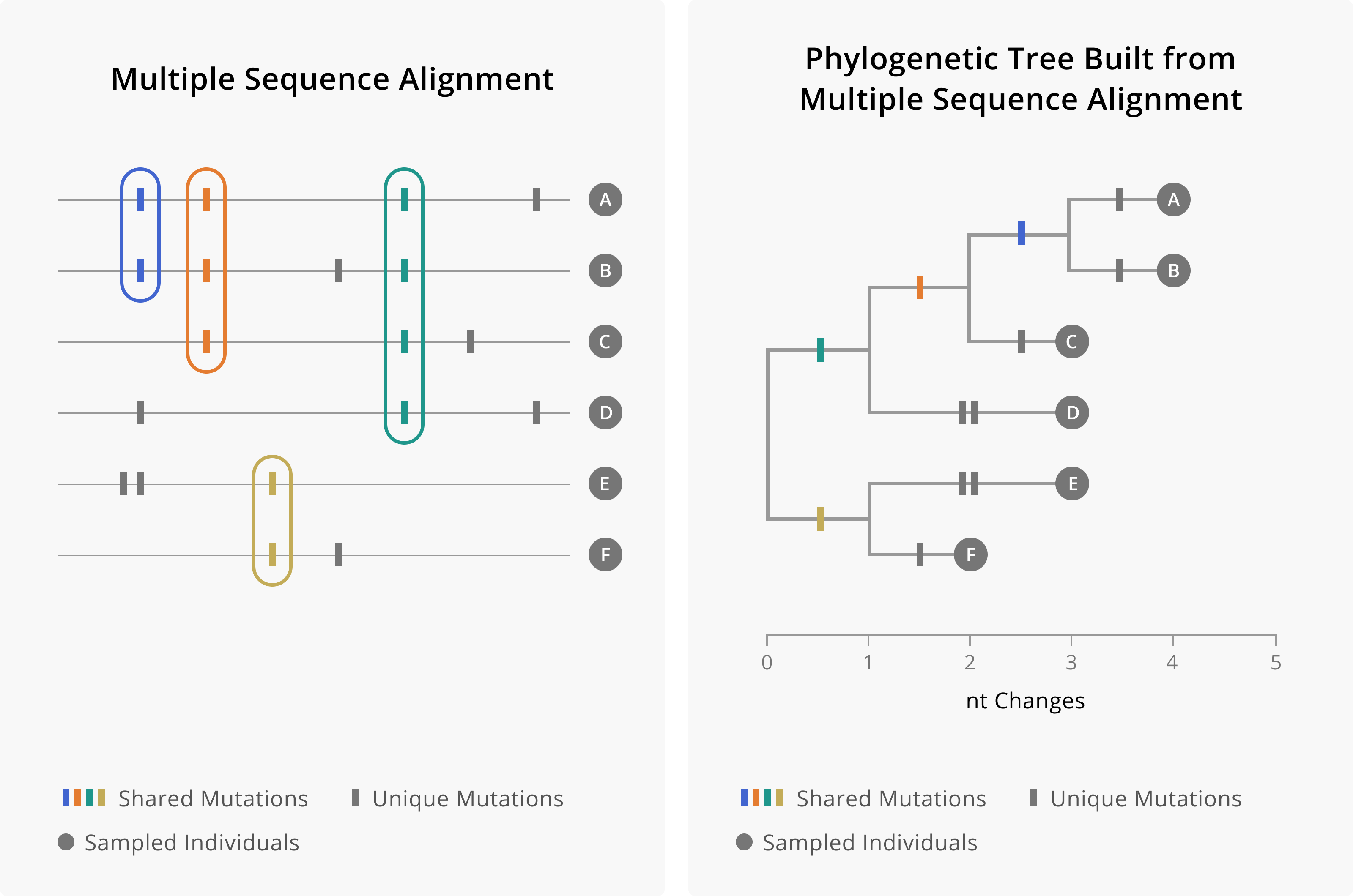
Figure 3.1: On the left is a theoretical multiple sequence alignment of genomes A through F. Shared mutations are found in multiple samples, while unique mutations are found only in one sampled sequence. We use this pattern of shared and unique mutations to build the phylogenetic tree, which hierarchically clusters tips according to which mutations they share. Mutations occur along branches, such that tips that descend from a branch will share that mutation. When mutations are shared by more samples, then those mutations would have occurred more deeply in the tree. Mutations that are unique to samples occur on external branches, whose only descendent is the sampled tip.
Within the phylogenetic tree, subgroups encompassing a common ancestor and all of its descendants are typically referred to as clades (or sometimes lineages). We define clades according to the mutations that the samples within the clade have inherited and all share. Clades are useful to consider when thinking about potentially altered biological properties. If a particular lineage has acquired novel mutations, and those mutations are passed on to its descendants, the entire clade would be expected to show the particular functional characteristics associated with the mutation(s) they all share.
Notably, because the phylogenetic clustering pattern is hierarchical, so are clades. Two sequences might cluster together into a small clade defined by a mutation that only they share. But those sequences can also be grouped within a larger clade, with additional samples, defined by a different set of mutations that occurred further back in the tree and were inherited by additional samples in the tree (Figure 3.2).
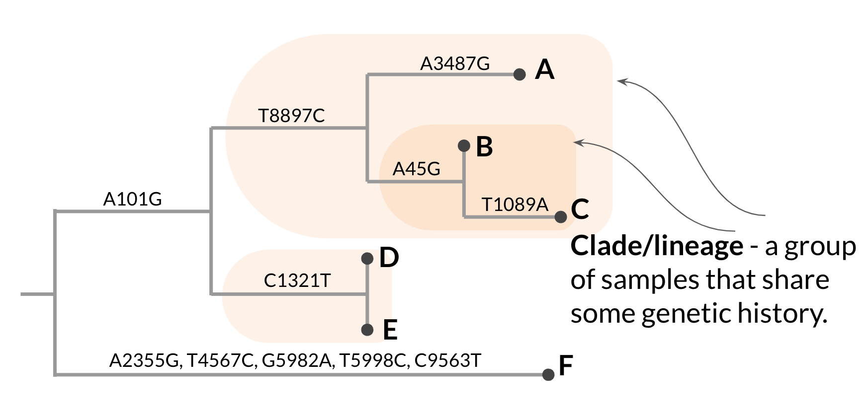
Figure 3.2: A hypothetical phylogenetic tree with hierarchical clades/lineages annotated.
It is common to encounter other embellishments on phylogenetic trees. For example, branches can be coloured to indicate inferred traits of ancestors in the tree. Common traits reconstructed on trees include geography or host. This annotation helps genomic epidemiologists understand the history and dynamics driving an epidemic. Another common addition, particularly to phylogenetic tree figures in scientific papers, are numbers or markers placed near or on nodes. These markers are a common way to indicate the statistical support for a given node (remember that each node is only a hypothesis of common descent). It has also become popular to mark mutations, particularly those changing amino acids in proteins, above the branch along which the mutations likely occurred.
It is common to encounter other embellishments on phylogenetic trees. For example, branches can be coloured to indicate inferred traits of ancestors in the tree. Common traits reconstructed on trees include geography or host. This annotation helps genomic epidemiologists understand the history and dynamics driving an epidemic. Another common addition, particularly to phylogenetic tree figures in scientific papers, are numbers or markers placed near or on nodes. These markers are a common way to indicate the statistical support for a given node (remember that each node is only a hypothesis of common descent). It has also become popular to mark mutations, particularly those changing amino acids in proteins, above the branch along which the mutations likely occurred.
Phylogenetic trees come in two categories: rooted and unrooted. An unrooted tree simply displays the inferred relationships between the samples without making any assumptions about where the tree begins. In contrast, rooted phylogenies explicitly state our hypothesis regarding the directionality of evolution. Within genomic epidemiology, you will primarily encounter rooted phylogenies, which is why we will concentrate on them in this section.
Within a rooted phylogeny, the direction of evolution proceeds from the root out towards the tips. Nodes that are basal in the tree, or deeper in the tree, are ancestral to nodes that are closer towards the tips (Figure 3.3). Rooted phylogenies are typically displayed in rectangular form, with the direction of evolution proceeding from the left to the right. In this format, the most basal node, the root, is the node that is furthest to the left, and descendants of that node will appear to the right of that node. That said, rooted phylogenies can be shown in other conformations as well, such as circular or top-to-bottom. In these cases, just remember that the direction of evolution proceeds from the root toward the tips. The branches are scaled in terms of genetic divergence, or the number of expected changes per nucleotide site.
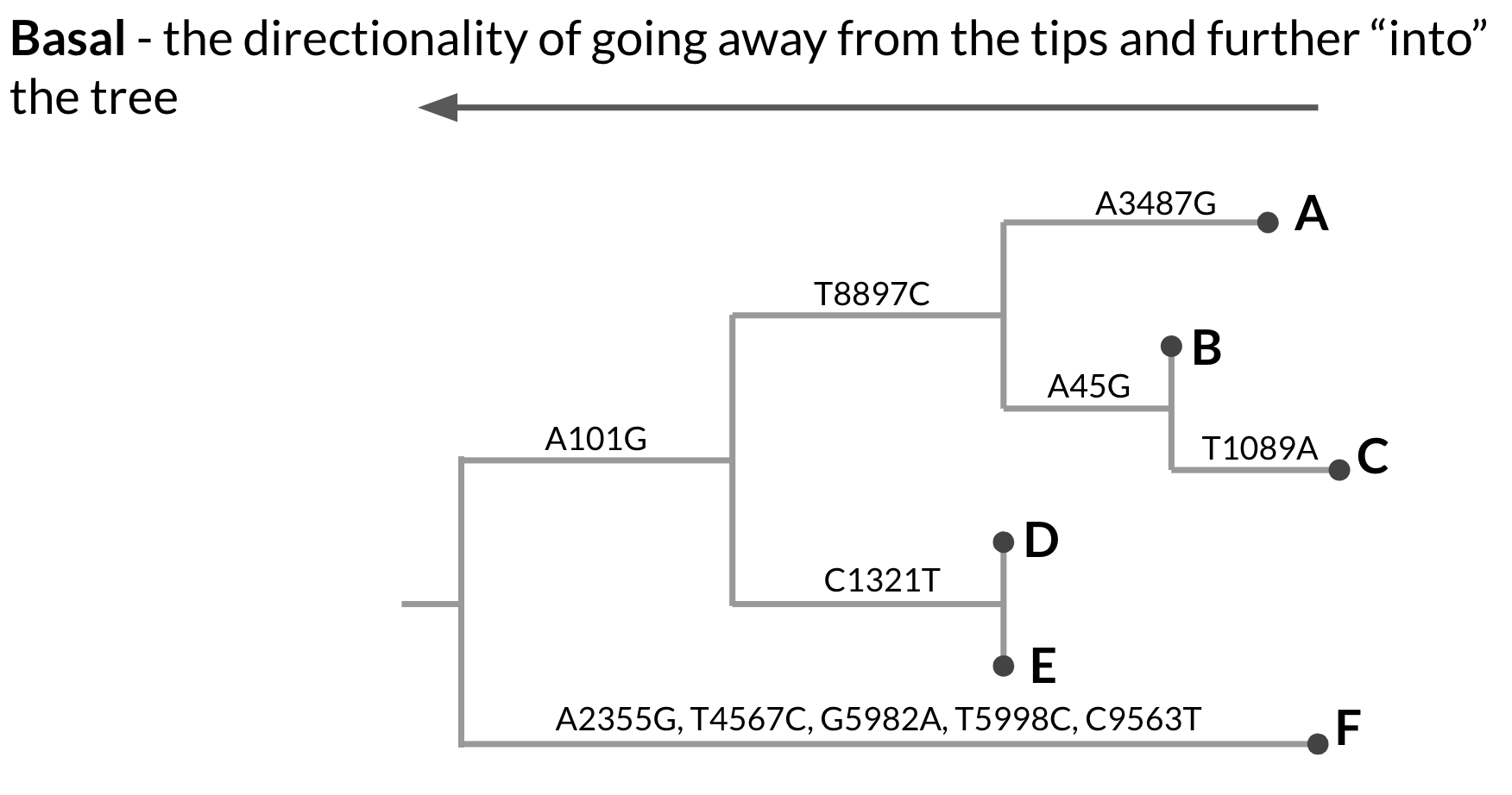
Figure 3.3: A hypothetical phylogenetic tree showing directionality. When we refer to a node being more basal within the tree, we mean deeper in the tree, closer to the root. The root is the most basal internal node in the tree. This phylogenetic tree is rectangular and oriented left-to-right. This means that the left-most internal node is the most basal, and the root, and that evolution proceeds forward from that node, moving from left-to-right.
3.5.2 Assessing and reading a phylogenetic tree.
Phylogenetic trees might seem simple, but correctly interpreting them is not always straightforward. For beginners and advanced users alike, interpreting a phylogenetic tree can present a challenge because the y-axis in a phylogenetic tree is meaningless. It is used to lay out all of the tips so they do not overlap - the proximity of any two tips along the y-axis does not indicate anything about their relatedness. This also means that the branching in a phylogeny can be rotated without altering the meaning of the diagram in any way. Because phylogenies sacrifice an entire dimension for clearly laying tips, there is also a limit on how much information can be packed into simple phylogenetic tree figures, and even moderately sized phylogenetic trees presented under ideal conditions can vary enormously in their ability to communicate key messages.
In learning how to assess a phylogenetic tree, we will consider only rooted phylogenetic trees, since you probably will not encounter scenarios where unrooted trees are necessary. One of the first things to check in a rooted tree is whether the root of the tree seems appropriate. The root of the tree represents the common ancestor of all your samples. Rooting determines the order of branching in the tree, and thus whether the root is correct or not will make all the difference when interpreting the tree. Ask yourself: “What lies on either side of the very first split in the tree?” You should be able to find a reference sequence representing the earliest known genome of a pathogen, or a fairly distinct but related organism (often termed an outgroup), or some known historical split in the pathogen’s population on one side of the root. Of course there are always caveats to this rule of thumb, but generally the rooting and directionality you observe in the tree should match your understanding of the pathogen’s descriptive epidemiology. Figure 3.4 below shows an example of how incorrectly rooting a phylogenetic tree can fundamentally, and incorrectly, alter your understanding of an evolutionary trajectory.
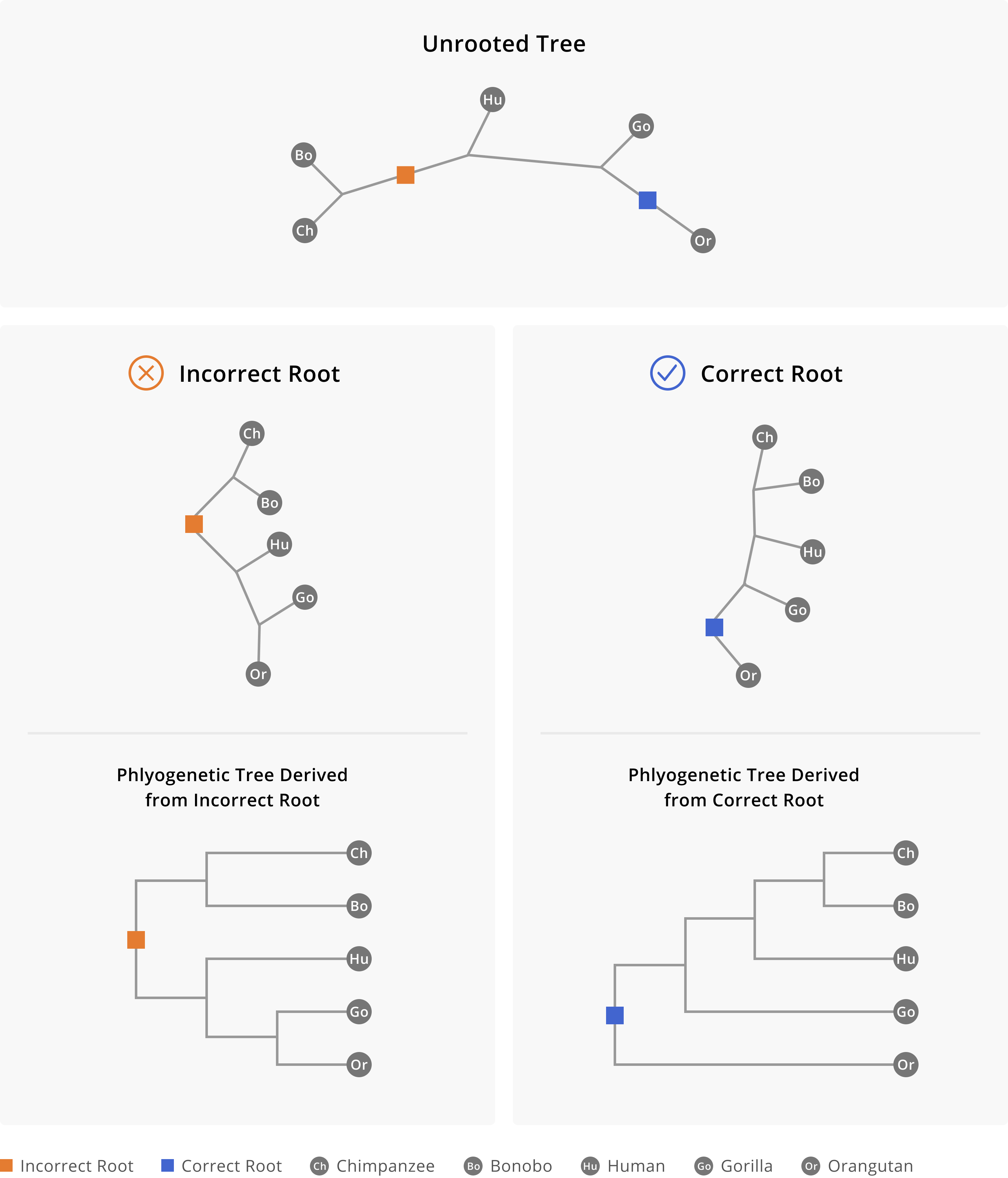
Figure 3.4: Rooting the phylogenetic tree of great apes. At the top we see the unrooted phylogeny, as well as two possible places we might place the root, one of which is correct and the other is incorrect. In selecting the root we describe a pattern of evolutionary descent out from the root. When the incorrect root is selected, on one side of the split we have chimpanzees and bonobos. On the other side of the split we have humans, gorillas, and orangutans. This does not match our understanding of evolutionary relationships between humans and great apes, and thus this particular split should alert us that the tree is incorrectly rooted. However, when the correct root is selected, as shown on the right hand side, we see a pattern of descent in which orangutans are on one side of the split, and chimpanzees, bonobos, humans, and gorillas are on the other side of the split. Chimpanzees and bonobos are most closely related to each other, followed by humans, then by gorillas.
Emanating from the root are branches representing direct lines of descent from the common ancestor. When looking at a genetic divergence phylogenetic tree, you will typically see that branch lengths are scaled in terms of a normalized number of substitutions per site in the genome. For increased interpretability, branches in genetic divergence trees may also be scaled in terms of total number of substitutions observed across the entire genome. Either way, both of these scalings represent an amount of sequence change that has occurred.
One thing to watch out for in genetic divergence phylogenies are particularly long branches, often at the tips. As discussed in the previous section, the length of a branch leading to a tip is scaled according to the number of mutations that are observed within that sample’s sequence, but not in other samples in the tree. If the numbers of mutations that are unique to a sample are very large, it is often an indicator of a sequence quality issue (for example, a sequencing error, or a bioinformatics issue with genome assembly).
3.5.3 Temporally-resolved phylogenetic trees.
The phylogenetic trees discussed thus far describe an inheritance process for the mutations observed in an alignment of sequences; these are genetic divergence phylogenetic trees. However, there is a second type of tree that you will commonly encounter in genomic epidemiology: temporally-resolved phylogenetic trees, also referred to as time trees.
Time trees make use of the molecular clock that we described earlier in this chapter to translate the amount of genetic divergence observed along branches of the tree into an estimate of the amount of calendar time that likely passed. This translation results in a tree where branch lengths are measured in absolute time rather than in genetic divergence. A few other shifts will occur in a time tree as well. Firstly, the position of the tips of the tree (those viruses that you have actually sampled and sequenced) is fixed at the date of sample collection, rather than representing how diverged a sample is from the root sequence. Secondly, the position of internal nodes in the tree is representative of when we think that ancestral node likely existed. The estimated date of an internal node in the tree comes from observing the sequence diversity of the descendents, and asking, “How far back in time would you need to go in order to find the common ancestor of these descendants?” This quantity is referred to as the time to the most recent common ancestor (TMRCA). For trees scaled in absolute time, it is not uncommon to indicate the range of uncertainty associated with the inferred date by providing a 95% confidence interval around the date. This may be given as a numerical range, or shown visually with a rectangle or a violin plot to show the full probability density.
Time trees have several useful properties that support epidemiological inference. Exploring trees along the dimension of time makes the tree more useful from a descriptive epidemiological perspective. For example, when we can move between genetic divergence trees and time trees, we can easily compare how the genomic diversity between samples aligns with the number of serial intervals separating sample collection dates. Furthermore, when we join information about sequenced samples (e.g. where they were collected) with information on when the common ancestors of those sequences likely circulated, we can begin to reconstruct when spatial movements of a pathogen occurred. This latter procedure is commonly referred to as phylogeography.
To discern whether you are looking at a time tree or a genetic divergence tree, look at the x-axis label or scale bar of your tree. If branch lengths are scaled in terms of absolute time (calendar time), then you have a time tree. Alternatively, if branch lengths are given in substitutions, or substitutions per site, then you are looking at a genetic divergence tree.
3.6 The transmission tree does not equate the phylogenetic tree.
Any branching process can be represented by tree-like graphs.The majority of this handbook discusses phylogenetic trees, which are hypotheses of common descent for genetic sequences. In such trees, sequenced cases at the tips of the tree are connected to inferred common ancestors, which may not have been directly observed. In contrast, within epidemiology we often think about transmission trees, in which nodes represent known cases, and edges connecting nodes represent the directionality of who-infected-whom. While it may seem like there are times when a network of who-infected-whom matches the phylogenetic tree, these two types of tree-like graphs are fundamentally different and should not be equated in practice.
What makes a phylogenetic tree different from a transmission tree? First and foremost, genetic mutations are not markers that a transmission event has occurred. Mutations occur spontaneously as the virus replicates, and this process is independent of whether the infection is passed on to another individual. While within-host diversity is sampled and passed on when a transmission event occurs, we do not always observe this variation at the consensus sequence level. As such, mutations in consensus genome sequences by no means occur with every single transmission event. Indeed, it is common for cases with direct epidemiologic linkage to have identical genome sequences.
Secondly, phylogenetic trees are inferred from sequences that are sampled from infected individuals at the time that a specimen is collected, not at the time that a transmission event occurs. This means that an observed sequence tells us something about that individual’s infection at the time that their specimen was collected, but not necessarily their infection at the time of a transmission event. Given that an individual’s within-host pathogen diversity is accumulating and changing over through the entire course of their infection, the sequence that summarizes diversity at the time of sample collection (the observable sequence) may not be identical to the sequence that summarizes within-host diversity at the time of transmission.
This issue is important because the sequence that is ancestral in a phylogenetic tree may not actually represent the infection that is ancestral. As a toy example, imagine a transmission event in which Person A infects Person B with some virus. Let’s say that Person A and Person B attended a party together just before Person A became symptomatic. Given this timing, Person A infected Person B early on in the course of their infection. However, Person A felt terrible, and didn’t seek testing until well into the course of their infection. In contrast, Person B heard that Person A was sick, and decided to seek testing just a couple of days after the party. In this scenario, despite Person A transmitting their infection to Person B, Person B’s diagnostic specimen is collected before Person A’s specimen is collected. Furthermore, given that Person B’s sample was collected early on in their infection, their sequence could be identical to the sequence that we would have observed from Person A had Person A got tested earlier. However, over the multiple days where Person A didn’t seek testing, they had further viral diversity accumulating, and by the time they finally get tested, the sequence characterizing their infection would have been additionally diverged.
In this case, it’s completely possible that while Person A truly did infect Person B, the viral genome sequence collected from Person B truly is ancestral to the sequence collected from Person A. In this way, an accurate portrayal of the pattern of genetic descent does not always show the exact directionality of transmission events.
Although sequencing cannot generally confirm who-infected-whom, there are exceptional cases where this is possible. Chronic viral infections, such as hepatitis C virus or HIV, have a great deal of time to accumulate diversity, making different individual’s infections very distinct. With appropriate sequencing methods that can capture this within-patient diversity, in both the infectee and the suspected infector, as well as community controls, it is possible to show that one individual’s viral diversity is a subset of another individual’s within-host diversity. Sequencing methods for accurately capturing within-host diversity tend to maximize sequencing depth and minimize errors. Public health applications typically do not sequence in this way for routine surveillance. However, such protocols are more common in academic studies, and are also used in court cases of criminal transmission.
3.7 Why is sequencing better at dismissing links than confirming them?
As we just discussed, observing mutations in consensus sequences is not a perfect marker of transmission events. As discussed at the beginning of this chapter, the power to use evolutionary analysis to explore epidemiological dynamics comes from the fact that changes to pathogen consensus genomes occur on similar timescales to transmission, but the two processes are not fundamentally joined together such that they occur at exactly the same time. This means that genomic data can provide greater resolution for understanding relationships between infections, but not perfect resolution.
The limits of using genomic data to resolve transmission dynamics are best observed for cases that are epidemiologically-linked, or closely-linked within a single transmission chain. Transmission among these cases, separated by one or only a few serial intervals, may have occurred faster than we see mutations arise within consensus sequences, leading to multiple cases with identical or highly similar consensus sequences.
This limitation imposes an important caveat to keep in mind as you perform genomic epidemiological inference; sequencing is generally better at dismissing epidemiologic linkage than confirming it.
Let’s walk through an example to illustrate this principle. Imagine you have two cases of a viral respiratory disease from the same household, with symptom onset dates roughly 3 days apart. Given the shared setting that these two people live in, and the timing of their infections, it seems likely that this pair of cases would represent an instance of household transmission, in which the case with the earlier symptom onset date likely infected the person with the later symptom onset date. Having genomic sequencing capacity in your public health lab, you take those two case’s diagnostic specimens and sequence the viral genomes. You look at the consensus genomes and see that despite these cases coming from the same household, the sequences are quite divergent from each other. Given the evolutionary rate of this respiratory virus, you estimate that you would need roughly 6 months worth of transmission to accumulate the total number of nucleotide differences observed between those two sequences. Furthermore, the two cases’ sequences are more related to other genome sequences collected in the area than they are to each other. You conclude that despite the shared living space and the timing of symptom onset, these two cases are not actually linked, and that it’s more probable that they were each independently infected in different settings outside the home. The divergence between their consensus genomes allows you to easily rule out linkage between them.
In contrast, imagine you take that same household pair, and they have identical genome sequences. Their infections are likely related, but you can’t tell from the genomic data who infected whom. Moreover, you can’t actually tell whether the transmission is even between these two cases. For instance, the household pair could both have been infected by a friend at a party they both attended, and they just had slightly different symptom onset rates. With identical genome sequences you can tell that the cases are likely related, but you often won’t know exactly how related, and it’s highly unlikely that you’ll be able to rule in a direct transmission event without pulling in additional sources of information.
3.7.1 How many mutations are enough to rule linkage out?
Coming back to ruling linkage out, what is the threshold at which there are “enough” mutations separating sequences that you can consider them to be unlinked? Like many things, the answer is “it depends”. And it depends on both the evolutionary rate of your pathogen of interest, and average length of the serial interval between two cases in a direct infection. Given that both these variables have distributions, it is best to think about sequence divergence and case linkage probabilistically. In the figures below we show probability distributions for whether cases are directly-linked given that their consensus genome sequences are separated by x mutations. We show these plots for two different (theoretical) viral pathogens with different evolutionary rates and different genome lengths to illustrate how thresholds can change depending on the pathogen and the rate of transmission.
In Figure 3.5 we imagine a viral pathogen with an evolutionary rate and genome length like pandemic H1N1 influenza. We show the probability that two cases are directly-linked given the number of mutations that separate two sequences. Each point in the plot represents a sample from the simulation, and the grey shaded areas represent the probability distributions given those samples. You can see that as the number of mutations separating sequences increases, the distribution of the probability that cases are linked decreases towards zero, but the distributions still have overlap. For instance, we still see that even when sequences are separated by two mutations, there is still a roughly 15% probability that the cases are linked. However, once you get to the point where the two sequences are separated by four or five mutations, there is an essentially zero percent probability that the cases are directly-linked.
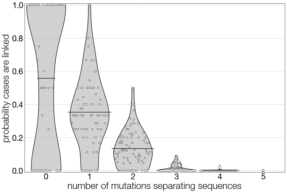
Figure 3.5: Probability distributions for whether cases are directly-linked, given their genomes are separated by a certain number of mutations. In this figure, the simulation from which these data are drawn recapitulates pandemic H1N1 influenza, with an evolutionary rate of 0.003406 substitutions per site per year, and a genome length of 13,154 nucleotides.
In Figure 3.6 we show the exact same procedure, however for a pathogen that is more SARS-CoV-2-like. Compared to pandemic H1N1 influenza, SARS-CoV-2 has a slightly slower evolutionary rate, but a genome that is more than twice as long. Comparing the two plots we can see that, with the second pathogen, the longer genome length (more sites where a mutation could occur) has provided us with a bit more resolution, and we can see that with more mutations separating two samples, the probability of linkage between the two cases drops off more quickly. That said, there continues to be overlap in the probability distributions, and you can see that there is still a non-negligible probability of direct linkage between cases whose sequences are separated by one mutation.
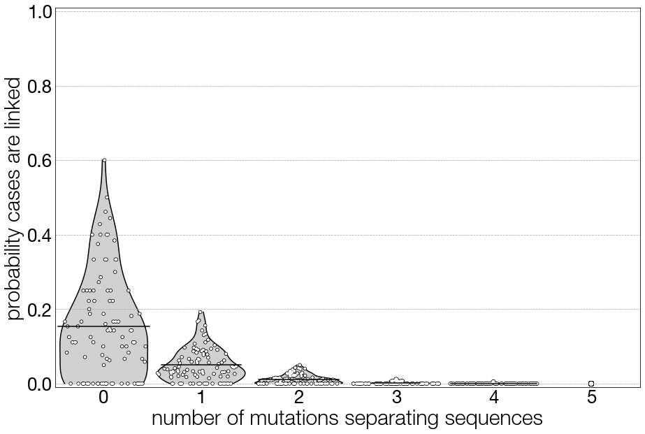
Figure 3.6: The same figure as above, but here the genomic parameters are SARS-CoV-2-like, with an evolutionary rate of 0.0008 substitutions per site per year and a genome length of 29,903 nucleotides.
In conclusion, we hope that these examples provide a clearer understanding of why it is easier to rule linkage out than it is to rule linkage in, and how to think probabilistically about linkage between cases given a certain level of sequence similarity. That said, we recommend that you use this information for shaping your interpretations of data, rather than setting an unvarying threshold by which you consider cases linked or unlinked. Many of the factors that go into shaping these plots are time-dependent. The average length of a serial interval between two linked-cases can rise and fall given changes to the number of individuals who remain susceptible and available to be infected, or the degree of superspreading that occurs, or changes to the intrinsic transmissibility of the pathogen. Furthermore, the evolutionary rates of the pathogens depend on various factors discussed in more depth earlier in this chapter. Taken together, this means that the similarity between the evolutionary timescale and transmission timescale can vary over an outbreak, even for the same pathogen. Thus, these principles should provide guidance and intuition for the data, but not enforce hard and fast thresholds.